A Quick Start Tutorial#

This tutorial provides a quick start guide to using ELISA to fit a spectral model to X-ray spectral data. The tutorial is divided into three sections:

Load Data and Define Spectral Model
Bayesian Fit
Maximum Likelihood Fit

The data used in this tutorial is from the Insight-HXMT observation of the Crab Nebula. The spectra are obtained by the Low Energy (LE), the Medium Energy (ME), and the High Energy (HE) telescopes. The spectral model used in this tutorial is a power-law model modified by a photoelectric absorption.

The tutorial demonstrates how to fit the spectral model to the data using both Bayesian and Maximum Likelihood methods.

1. Load Data and Define Spectral Model#

from elisa import BayesFit, Data, MaxLikeFit
from elisa.models import PhAbs, PowerLaw

LE = Data(
    erange=[1.5, 10],
    specfile='data/P011160500104_LE.pi',
    backfile='data/P011160500104_LE.bak',
    respfile='data/P011160500104_LE.rsp',
    group='opt',
)

ME = Data(
    erange=[10, 35],
    specfile='data/P011160500104_ME.pi',
    backfile='data/P011160500104_ME.bak',
    respfile='data/P011160500104_ME.rsp',
    group='opt',
)

HE = Data(
    erange=[28, 250],
    specfile='data/P011160500104_HE.pi',
    backfile='data/P011160500104_HE.bak',
    respfile='data/P011160500104_HE.rsp',
    group='opt',
)

data = [LE, ME, HE]

model = PhAbs() * PowerLaw()

/home/docs/checkouts/readthedocs.org/user_builds/astro-elisa/conda/v0.2.3/lib/python3.12/site-packages/elisa/util/config.py:80: Warning: only 2 CPUs available, will use 1 CPUs
  warnings.warn(msg, Warning)
/tmp/ipykernel_3307/205821572.py:4: Warning: spectrum data/P011160500104_LE.bak has zero statistical errors, which may lead to wrong result under Gaussian statistics, consider grouping the spectrum
  LE = Data(

/tmp/ipykernel_3307/205821572.py:12: Warning: spectrum data/P011160500104_ME.bak has zero statistical errors, which may lead to wrong result under Gaussian statistics, consider grouping the spectrum
  ME = Data(
/tmp/ipykernel_3307/205821572.py:20: Warning: spectrum data/P011160500104_HE.bak has zero statistical errors, which may lead to wrong result under Gaussian statistics, consider grouping the spectrum
  HE = Data(

2. Bayesian Fit#

fit = BayesFit(data, model)
fit

Bayesian Fit

Data	Model	Statistic
LE	PhAbs * PowerLaw	pgstat
ME	PhAbs * PowerLaw	pgstat
HE	PhAbs * PowerLaw	pgstat

No.	Component	Parameter	Value	Prior
1	PhAbs	nH	1	Uniform(0, 1e+06)
2	PowerLaw	alpha	1.01	Uniform(-3, 10)
3	PowerLaw	K	1	Uniform(1e-10, 1e+10)

Run the No-U-Turn Sampler#

posterior = fit.nuts(progress=False)
posterior

/home/docs/checkouts/readthedocs.org/user_builds/astro-elisa/conda/v0.2.3/lib/python3.12/site-packages/arviz/stats/stats.py:1652: UserWarning: For one or more samples the posterior variance of the log predictive densities exceeds 0.4. This could be indication of WAIC starting to fail. 
See http://arxiv.org/abs/1507.04544 for details
  warnings.warn(

Posterior Result

Parameters

Parameter	Mean	StdDev	Median	68.3% Quantile	ESS	Rhat
PhAbs.nH	0.355	0.0092	0.355	[-0.00924, 0.00945]	1803	N/A
PowerLaw.alpha	2.12	0.0022	2.12	[-0.00227, 0.00212]	2017	N/A
PowerLaw.K	8.9	0.0461	8.9	[-0.0476, 0.046]	1856	N/A

Statistics

Data	Statistic	Mean	Median	Channels
LE	pgstat	122.14	121.56	96
ME	pgstat	18.00	17.56	17
HE	pgstat	30.65	30.04	28
Total	stat/dof	170.80/138	170.18/138	141

Information Criterion

Method	Deviance	p
LOOIC	175.20 ± 22.77	4.15
WAIC	175.15 ± 22.76	4.12

Pareto k Diagnostic

Range	Flag	Count	Pct.
(-Inf, 0.70]	good	141	100.0%
(0.70, 1]	bad	0	0.0%
(1, Inf)	very bad	0	0.0%

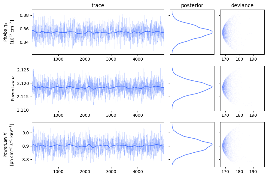
Plot the Trace of Sampler#

fig = posterior.plot.plot_trace()

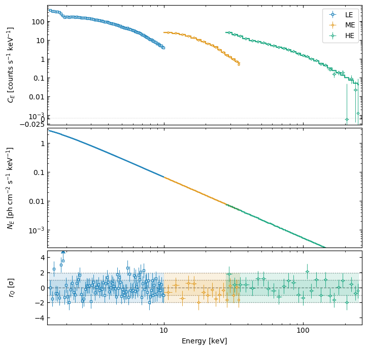
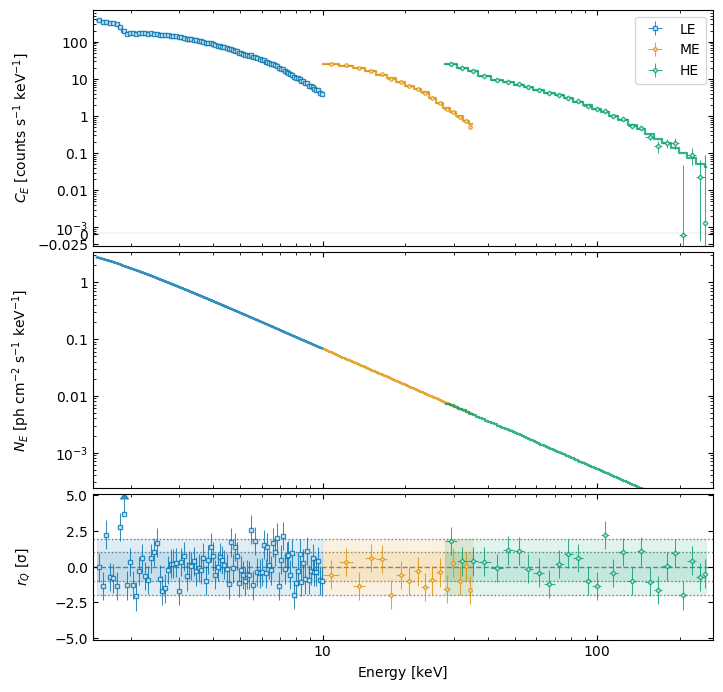
../_images/d591a354b48854fa95f3b8b958802e4e2dcde5d9cf09df903e8362587858c32d.png

Plot of Spectral Fit and Residuals#

fig = posterior.plot()

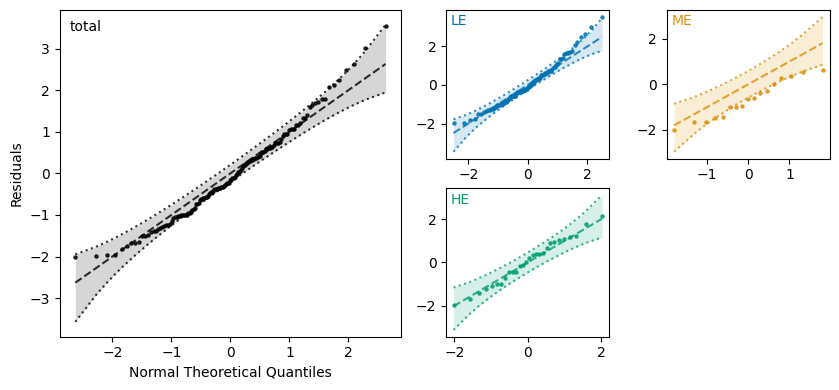
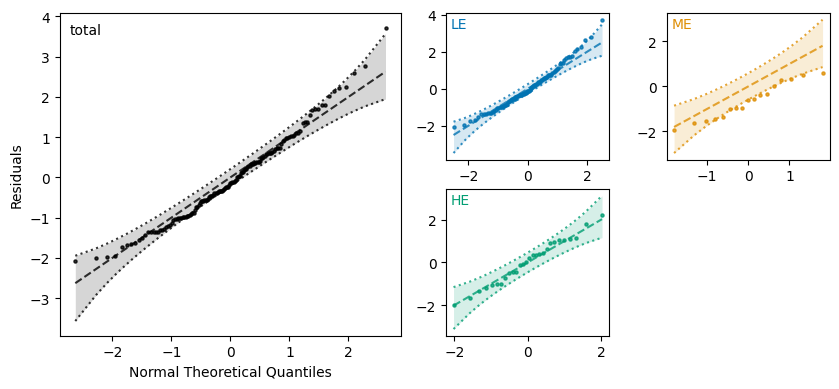
../_images/f195bdbe5df902630976a7c9c85a85763b64ea01ca9cf12ef75e8fe74e999ecc.png

Goodness of Fit: Quantile-Quantile Plot#

fig = posterior.plot.plot_qq(detrend=False)

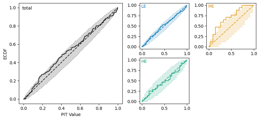
../_images/0f0db8790a54cb1b960e46ad43368c680d8e7a1d73cbb558b21cc4c331e1a64c.png

Goodness of Fit: Probability Integral Transform ECDF Plot#

fig = posterior.plot.plot_pit(detrend=False)

../_images/068d6741ca59375c0425efa7b45b14e435d3d572701422803dc699e48a953560.png

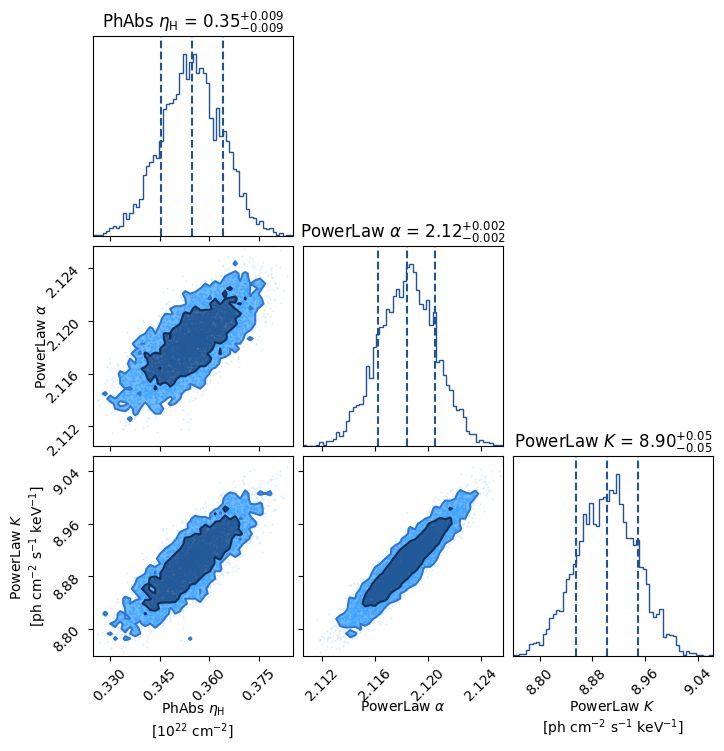
Plot Marginal Posterior Distribution#

fig = posterior.plot.plot_corner()

../_images/5ee03ef54cf3883a64e6785696b863dc055562695fd72287516709a30026d3bd.png

Calculate Credible Intervals of Parameters#

ci = posterior.ci()
ci

CredibleInterval(median={'PhAbs.nH': 0.35468305783170384, 'PowerLaw.alpha': 2.118439713044811, 'PowerLaw.K': 8.902595929877329}, intervals={'PhAbs.nH': (0.345448912867953, 0.3641243930036606), 'PowerLaw.alpha': (2.116175518266008, 2.1205576309978933), 'PowerLaw.K': (8.854995319667175, 8.948625836633322)}, errors={'PhAbs.nH': (-0.009234144963750857, 0.009441335171956777), 'PowerLaw.alpha': (-0.0022641947788031302, 0.002117917953082138), 'PowerLaw.K': (-0.047600610210153604, 0.04602990675599372)}, cl=np.float64(0.6826894921370859), method='ETI', dist={'PhAbs.nH': array([[0.35307594, 0.35265833, 0.35399535, ..., 0.36013947, 0.36016573,
        0.35814949]], shape=(1, 5000)), 'PowerLaw.alpha': array([[2.12020645, 2.12094415, 2.11882787, ..., 2.11864643, 2.12070248,
        2.11706934]], shape=(1, 5000)), 'PowerLaw.K': array([[8.93632502, 8.94852556, 8.9081469 , ..., 8.93408391, 8.92631465,
        8.87832211]], shape=(1, 5000))})

ci.median

{'PhAbs.nH': 0.35468305783170384,
 'PowerLaw.alpha': 2.118439713044811,
 'PowerLaw.K': 8.902595929877329}

ci.errors

{'PhAbs.nH': (-0.009234144963750857, 0.009441335171956777),
 'PowerLaw.alpha': (-0.0022641947788031302, 0.002117917953082138),
 'PowerLaw.K': (-0.047600610210153604, 0.04602990675599372)}

3. Maximum Likelihood Fit#

model.PhAbs.nH.default = 0.35
fit2 = MaxLikeFit([LE, ME, HE], model)
fit2

Maximum Likelihood Fit

Data	Model	Statistic
LE	PhAbs * PowerLaw	pgstat
ME	PhAbs * PowerLaw	pgstat
HE	PhAbs * PowerLaw	pgstat

No.	Component	Parameter	Value	Bound
1	PhAbs	nH	0.35	(0, 1e+06)
2	PowerLaw	alpha	1.01	(-3, 10)
3	PowerLaw	K	1	(1e-10, 1e+10)

Use Levenberg-Marquardt algorithm to find the MLE#

mle = fit2.mle(method='lm')
mle

MLE Result

Parameters

Parameter	MLE	Error
PhAbs.nH	0.3543	0.009225
PowerLaw.alpha	2.118	0.002194
PowerLaw.K	8.9	0.0461

Fit Statistics

Data	Statistic	Value	Channels
LE	pgstat	120.24	96
ME	pgstat	17.62	17
HE	pgstat	29.97	28
Total	stat/dof	167.83/138	141

Information Criterion

Method	Value
AIC	174.00
BIC	182.67

Fit Status

Migrad
FCN = 167.8 (χ²/ndof = 1.2)	Nfcn = 98, Ngrad = 1
EDM = 2.3e-08 (Goal: 0.0002)	time = 3.2 sec
Valid Minimum	Below EDM threshold (goal x 10)
No parameters at limit	Below call limit
Hesse ok	Covariance accurate

Plot of Spectral Fit and Residuals#

fig = mle.plot()

../_images/36157348f00c5513c6d6a19cdd56d89246d30e46cb7f0363babb799030de758a.png

Goodness of Fit: Quantile-Quantile Plot#

fig = mle.plot.plot_qq(detrend=False)

../_images/c8b74d0fab0ee0f173093518df7c79480922cdd19200156379b583b19989506e.png

Goodness of Fit: Probability Integral Transform ECDF Plot#

fig = mle.plot.plot_pit(detrend=False)

../_images/02fba5bb86e4d51b32893930aaf03260a10a10532e42c50673a0957164d4ad90.png

Calculate Confidence Intervals of Parameters#

ci = mle.ci()
ci

ConfidenceInterval(mle={'PhAbs.nH': 0.35429926252127875, 'PowerLaw.alpha': 2.1183203931005345, 'PowerLaw.K': 8.899948343483342}, se={'PhAbs.nH': 0.00922543955714701, 'PowerLaw.alpha': 0.002193915753357573, 'PowerLaw.K': 0.04610361194426487}, intervals={'PhAbs.nH': (0.3450776689087919, 0.36352855437839926), 'PowerLaw.alpha': (2.1161287517819476, 2.1205165866293942), 'PowerLaw.K': (8.8539784987533, 8.94618633190051)}, errors={'PhAbs.nH': (-0.009221593612486867, 0.009229291857120514), 'PowerLaw.alpha': (-0.0021916413185869565, 0.002196193528859691), 'PowerLaw.K': (-0.04596984473004184, 0.046237988417168197)}, cl=np.float64(0.6826894921370859), method='profile', status={'PowerLaw.K': {'valid': (True, True), 'at_limit': (False, False), 'at_max_fcn': (False, False), 'new_min': (False, False)}, 'PowerLaw.alpha': {'valid': (True, True), 'at_limit': (False, False), 'at_max_fcn': (False, False), 'new_min': (False, False)}, 'PhAbs.nH': {'valid': (True, True), 'at_limit': (False, False), 'at_max_fcn': (False, False), 'new_min': (False, False)}})

ci.mle

{'PhAbs.nH': 0.35429926252127875,
 'PowerLaw.alpha': 2.1183203931005345,
 'PowerLaw.K': 8.899948343483342}

ci.errors

{'PhAbs.nH': (-0.009221593612486867, 0.009229291857120514),
 'PowerLaw.alpha': (-0.0021916413185869565, 0.002196193528859691),
 'PowerLaw.K': (-0.04596984473004184, 0.046237988417168197)}