Model Building

The modeling framework of ELISA is designed to be flexible, allowing you to construct arbitrarily complex models by combining models from ELISA or XSPEC, as well as your custom models. Links between parameters across different model components can also be established. These models can then be fitted to the spectral datasets.

The Model Interface

In the context of X/\(\gamma\)-ray spectral fitting, a spectral model is a photon flux model. The model may be composed by a single flux component, or many additive flux components, and these additive components can be further modified by multiplicative or convolution components. You can check ELISA’s built-in model components from the API Reference:

• additive

• multiplicative

• convolution

Create a Model

To use the spectral models in ELISA, you can run the following code to import all model classes of three types from the elisa.models module:

from elisa.models import *

/home/docs/checkouts/readthedocs.org/user_builds/astro-elisa/conda/latest/lib/python3.12/site-packages/elisa/util/config.py:82: Warning: only 2 CPUs available, will use 1 CPUs
  warnings.warn(msg, Warning)

After the import, you can create an instance of a model by calling the model class. For example, the following code creates a PowerLaw photon flux model:

m = PowerLaw()
m

Additive Model: PowerLaw

No.	Component	Parameter	Value	Bound	Prior
1	PowerLaw	alpha	1.01	(-3, 10)	Uniform(-3, 10)
2	PowerLaw	K	1	(1e-10, 1e+10)	Uniform(1e-10, 1e+10)

The string representation of the model shows its name along with its model type, the components and corresponding parameters. We can see that the parameters are initialized with default values, bounds, and the prior distribution. We will discuss how to configure the default values, bounds, and priors of these parameters in the parameter interface section.

Next, we can create a new model by modifying the power-law model with a photoelectric absorption component PhAbs. We first create the absorption model along with the angr abundance table and the vern photoelectric cross-section.

phabs = PhAbs(abund='angr', xsect='vern')
phabs

Multiplicative Model: PhAbs

No.	Component	Parameter	Value	Bound	Prior
1	PhAbs	nH	1	(0, 1e+06)	Uniform(0, 1e+06)

Note that PhAbs uses angr abundance and vern cross-section by default, and thus PhAbs(abund='angr', xsect='vern') is equivalent to PhAbs().

Then, we can create a new model by multiplying the power-law model with the photoelectric absorption component:

m2 = phabs * PowerLaw()
m2

Additive Model: PhAbs * PowerLaw

No.	Component	Parameter	Value	Bound	Prior
1	PhAbs	nH	1	(0, 1e+06)	Uniform(0, 1e+06)
2	PowerLaw	alpha	1.01	(-3, 10)	Uniform(-3, 10)
3	PowerLaw	K	1	(1e-10, 1e+10)	Uniform(1e-10, 1e+10)

Assume the model is for an extragalactic source with a redshift measurement like \(z=1.5\), we convolve the photon flux model with ZAShift to account for the redshift. We first create the redshift component,

redshift = ZAShift(z=1.5)
redshift

Convolution Model: ZAShift

No.	Component	Parameter	Value	Bound	Prior
	ZAShift	z	1.5

We can see that the redshift parameter is fixed to 1.5. Now we can create a new model by convolving the previous model with the redshift component:

m3 = redshift(m2)
m3

Additive Model: ZAShift(PhAbs * PowerLaw)

No.	Component	Parameter	Value	Bound	Prior
1	PhAbs	nH	1	(0, 1e+06)	Uniform(0, 1e+06)
2	PowerLaw	alpha	1.01	(-3, 10)	Uniform(-3, 10)
3	PowerLaw	K	1	(1e-10, 1e+10)	Uniform(1e-10, 1e+10)
	ZAShift	z	1.5

The model is now a power-law model with photoelectric absorption, and further modified by the redshift.

Note that the same model can be created with a single line code:

m4 = ZAShift(z=1.5)(PhAbs() * PowerLaw())
m4

Additive Model: ZAShift(PhAbs * PowerLaw)

No.	Component	Parameter	Value	Bound	Prior
1	PhAbs	nH	1	(0, 1e+06)	Uniform(0, 1e+06)
2	PowerLaw	alpha	1.01	(-3, 10)	Uniform(-3, 10)
3	PowerLaw	K	1	(1e-10, 1e+10)	Uniform(1e-10, 1e+10)
	ZAShift	z	1.5

Now let’s have a look at the spectral shape of the model we just built,

import matplotlib.pyplot as plt
import numpy as np

plt.rcParams['axes.formatter.min_exponent'] = 3

# Compile the model and get CompiledModel instance
compiled_model = m4.compile()

# Create a photon energy grid used to evaluate the model
photon_egrid = np.linspace(0.3, 15.0, 1000)
egrid_mid = 0.5 * (photon_egrid[:-1] + photon_egrid[1:])

# Evaluate the model with the default parameters
# photon flux N(E) [s^-1 cm^-2 keV^-1]
ne = compiled_model.ne(photon_egrid)

# You can also evaluate the model with custom
# parameters, by specifying either a full set
# or a subset of parameters to CompiledModel.ne
custom_params = {'PowerLaw.alpha': 2.0}
ne2 = compiled_model.ne(photon_egrid, params=custom_params)

ne3 = compiled_model.ne(photon_egrid, params={'ZAShift.z': 0.0})

# For Fv or vFv plot, we can use ene and eene
# ene = compiled_model.ene(photon_egrid)
# eene = compiled_model.eene(photon_egrid)

plt.step(egrid_mid, ne, label='default')
plt.step(egrid_mid, ne2, label='alpha=2.0')
plt.step(egrid_mid, ne3, label='z=0.0')
plt.legend()
plt.title(m4.name)
plt.xlabel('Energy [keV]')
plt.ylabel('$N_E$ [ph cm$^{-2}$ s$^{-1}$ keV$^{-1}$]')
plt.xscale('log')
plt.yscale('log')

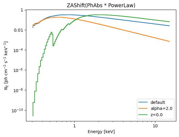
Great! We have successfully built a model and inspected its spectral shape. You can build any model you want in a similar way.

Tip

The model’s \(F_\nu\) and \(\nu F_\nu\) values can be accessed by CompiledModel’s ene and eene methods.

In addition, CompiledModel provides tools to calculate flux, isotropic-equivalent luminosity and energy.

Use XSPEC Models

ELISA can make use of XSPEC models. Before using them, you need to follow the Installation Guide to install the xspex package, which provides JAX interface for XSPEC models.

Once xspex package is installed successfully, import ELISA’s wrapper of XSPEC models by

from elisa.models import xs

failed to resolve latest value for ATOMDB_VERSION: "/home/docs/checkouts/readthedocs.org/user_builds/astro-elisa/conda/latest/heasoft/../spectral/modelData/latest.txt" is missing and Xspec.init does not provide a concrete versionfailed to resolve latest value for SPEX_VERSION: "/home/docs/checkouts/readthedocs.org/user_builds/astro-elisa/conda/latest/heasoft/../spectral/modelData/latest.txt" is missing and Xspec.init does not provide a concrete versionfailed to resolve latest value for NEI_VERSION: "/home/docs/checkouts/readthedocs.org/user_builds/astro-elisa/conda/latest/heasoft/../spectral/modelData/latest.txt" is missing and Xspec.init does not provide a concrete version

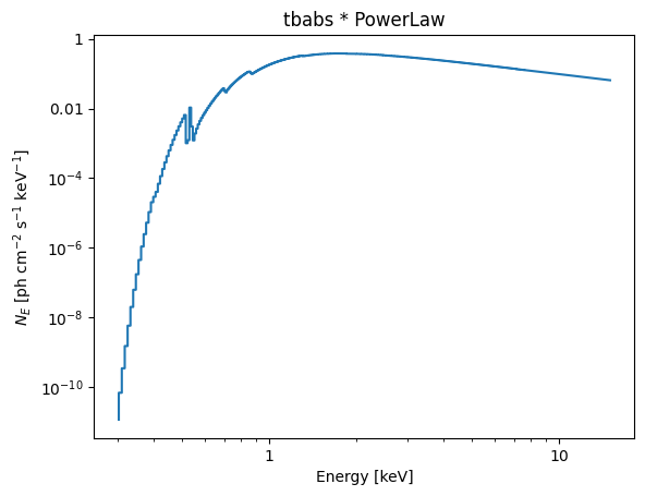
We can build a model combining models from both ELISA and XSPEC. For examle,

xs.abund('wilm')  # set the abundance table to wilm for tbabs
m5 = xs.tbabs() * PowerLaw()
m5

 Solar Abundance Vector set to wilm:  Wilms, J., Allen, A. & McCray, R. ApJ 542 914 (2000) (abundances are set to zero for those elements not included in the paper).

Additive Model: tbabs * PowerLaw

No.	Component	Parameter	Value	Bound	Prior
1	tbabs	nH	1	(0, 1e+06)	Uniform(0, 1e+06)
2	PowerLaw	alpha	1.01	(-3, 10)	Uniform(-3, 10)
3	PowerLaw	K	1	(1e-10, 1e+10)	Uniform(1e-10, 1e+10)

photon_egrid = np.linspace(0.3, 15.0, 2000)
egrid_mid = 0.5 * (photon_egrid[:-1] + photon_egrid[1:])
ne = m5.compile().ne(photon_egrid)
plt.step(egrid_mid, ne)
plt.title(m5.name)
plt.xlabel('Energy [keV]')
plt.ylabel('$N_E$ [ph cm$^{-2}$ s$^{-1}$ keV$^{-1}$]')
plt.xscale('log')
plt.yscale('log')

m6 = xs.thcomp()(PowerLaw())
m6

/home/docs/checkouts/readthedocs.org/user_builds/astro-elisa/conda/latest/lib/python3.12/site-packages/elisa/models/parameter.py:637: Warning: the default value of cov_frac (1.0) is equal to its max (1.0), which will lead to undefined result; the default value is now reset to 0.9999999999
  warnings.warn(

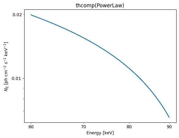
Additive Model: thcomp(PowerLaw)

No.	Component	Parameter	Value	Bound	Prior
1	PowerLaw	alpha	1.01	(-3, 10)	Uniform(-3, 10)
2	PowerLaw	K	1	(1e-10, 1e+10)	Uniform(1e-10, 1e+10)
3	thcomp	Gamma_tau	1.7	(1.001, 10)	Uniform(1.001, 10)
4	thcomp	kT_e	50	(0.5, 150)	Uniform(0.5, 150)
5	thcomp	cov_frac	1	(0, 1)	Uniform(0, 1)
	thcomp	z	0

photon_egrid = np.linspace(60.0, 90.0, 1000)
egrid_mid = 0.5 * (photon_egrid[:-1] + photon_egrid[1:])
ne = m6.compile().ne(photon_egrid)
plt.step(egrid_mid, ne)
plt.title(m6.name)
plt.xlabel('Energy [keV]')
plt.ylabel('$N_E$ [ph cm$^{-2}$ s$^{-1}$ keV$^{-1}$]')
plt.xscale('log')
plt.yscale('log')

Use Custom Models

You can also include custom models when building models. See Make Custom Models tutorial for details on how to make a custom model.

Conclusion

By leveraging the model interface of ELISA, you can construct arbitrarily complex spectral models to suit your needs.

In the next section, we will discuss the parameter configuration for the model.

The Parameter Interface

ELISA provide an intuitive way to configure the parameters of the model components.

As we have seen in the previous section, the model components have parameters associated with them. These parameters have default values, bounds, and prior distributions defined. Indeed, these parameters are instances of the Parameter class.

The Uniform Parameter

When creating a model without specifying the configuration of parameters, UniformParameter instances are automatically created and assigned to model components.

For example, when we initialize a PowerLaw simply by PowerLaw(), information is read from the PowerLaw._config attribute and passed to the UniformParameter to create the parameter objects for the power-law model. The information includes the default values, bounds, and flags to indicate whether the parameters are parameterized in logarithmic space and whether to be fixed. This is also the case for other model components.

for i in PowerLaw._config:
    print(i, end='\n\n')

ParamConfig(name='alpha', latex='\\alpha', unit='', default=1.01, min=-3.0, max=10.0, log=False, fixed=False)

ParamConfig(name='K', latex='K', unit='ph cm^-2 s^-1 keV^-1', default=1.0, min=1e-10, max=10000000000.0, log=False, fixed=False)

PowerLaw()

Additive Model: PowerLaw

No.	Component	Parameter	Value	Bound	Prior
1	PowerLaw	alpha	1.01	(-3, 10)	Uniform(-3, 10)
2	PowerLaw	K	1	(1e-10, 1e+10)	Uniform(1e-10, 1e+10)

We can see that the configuration of parameters matches the information printed above.

Usually, it is fine to use the default configuration. However, you can customize the parameters for your need. For example, you can create UniformParameter instances with custom default values and bounds, and then passed to the model constructor:

from elisa import UniformParameter

alpha = UniformParameter(
    name='alpha', default=2.0, min=0.0, max=5.0, log=False, fixed=False
)

K = UniformParameter(
    name='K', default=10, min=1e-5, max=1e5, log=True, fixed=False
)

PowerLaw(alpha=alpha, K=K)

Additive Model: PowerLaw

No.	Component	Parameter	Value	Bound	Prior
1	PowerLaw	alpha	2	(0, 5)	Uniform(0, 5)
2	PowerLaw	K	10	(1e-05, 1e+05)	LogUniform(1e-05, 1e+05)

ELISA also provides several convenient ways to set up the UniformParameter for model components, without the need to create the UniformParameter instances explicitly:

Passing size one float sequence to the model constructor will create a UniformParameter with the float as the default value,

PowerLaw(alpha=[1.7])

Additive Model: PowerLaw

No.	Component	Parameter	Value	Bound	Prior
1	PowerLaw	alpha	1.7	(-3, 10)	Uniform(-3, 10)
2	PowerLaw	K	1	(1e-10, 1e+10)	Uniform(1e-10, 1e+10)

Passing three-sequence will create a UniformParameter with the first element as the default value, the second and third elements as the minimum and maximum values,

Blackbody(kT=(10, 2, 30), K=[1.1, 1e-5, 1e4])

Additive Model: Blackbody

No.	Component	Parameter	Value	Bound	Prior
1	Blackbody	kT	10	(2, 30)	Uniform(2, 30)
2	Blackbody	K	1.1	(1e-05, 1e+04)	Uniform(1e-05, 1e+04)

Passing a four-sequence will create a UniformParameter with the first three elements as the default, minimum and maximum values, and the fourth element as the flag to indicate whether the parameter is logarithmically parameterized,

TBAbs(nH=[3.0, 0.01, 10.0, True])

Multiplicative Model: TBAbs

No.	Component	Parameter	Value	Bound	Prior
1	TBAbs	nH	3	(0.01, 10)	LogUniform(0.01, 10)

And finally, passing a float will create a UniformParameter with the float as the default value, and the parameter is fixed to this value,

ZAShift(z=4.2)

Convolution Model: ZAShift

No.	Component	Parameter	Value	Bound	Prior
	ZAShift	z	4.2

Other Parameters

In addition to the UniformParameter, ELISA provides three other types of parameters.

DistParameter

You can create a DistParameter instance by passing a NumPyro’s probability distribution instance. This is useful when you want to use non-uniform priors for parameters in Bayesian analysis. For example, we can create a multiplicative Constant component with a Gaussian prior in \(\mathbb{R^+}\).

import numpyro.distributions as dist

from elisa import DistParameter

f = DistParameter(
    name='f',
    dist=dist.TruncatedNormal(
        loc=1.0,
        scale=0.2,
        low=0.0,
    ),
    default=1.0,
)
Constant(f=f)

Multiplicative Model: Constant

No.	Component	Parameter	Value	Bound	Prior
1	Constant	f	1	GreaterThan(lower_bound=0.0)	LeftTruncatedDistribution(low=0)

ConstantInterval

When assigning ConstantInterval parameters to a model component, the model will be evaluated according to the following formula:

\[\frac{1}{\prod_i (b_i - a_i)} \int f(E, \vec{\theta}(\vec{p}, \vec{q})) \, \mathrm{d} \vec{p}\]

where \(f\) is the model function, \(\vec{\theta}\) is the parameter vector of the model, \(\vec{p}\) is the ConstantInterval parameters, \(\vec{q}\) is the other parameters, and \(a_i\) and \(b_i\) are the intervals given by \(\vec{p}\).

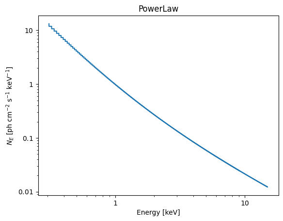
from elisa import ConstantInterval

alpha = ConstantInterval(
    name='alpha',
    interval=[1.0, 3.0],
)
m7 = PowerLaw(alpha=alpha)
m7

Additive Model: PowerLaw

No.	Component	Parameter	Value	Bound	Prior
	PowerLaw	alpha	[1, 3]
1	PowerLaw	K	1	(1e-10, 1e+10)	Uniform(1e-10, 1e+10)

photon_egrid = np.linspace(0.3, 15.0, 1000)
egrid_mid = 0.5 * (photon_egrid[:-1] + photon_egrid[1:])
ne = m7.compile().ne(photon_egrid)
plt.step(egrid_mid, ne)
plt.title(m7.name)
plt.xlabel('Energy [keV]')
plt.ylabel('$N_E$ [ph cm$^{-2}$ s$^{-1}$ keV$^{-1}$]')
plt.xscale('log')
plt.yscale('log')

CompositeParameter

CompositeParameter combines multiple parameters into a single parameter. The value of the composite parameter is calculated by a user-defined function that takes the values of the constituent parameters as input. Note that the function must be JAX compatible.

It is the key for linking parameters across different model components. For example, we can create a double Blackbody model, forcing the temperature of one component to be smaller than that of the other,

import jax.numpy as jnp

from elisa import CompositeParameter

# Define the temperature parameter of the first blackbody
kT1 = UniformParameter(
    name='kT',
    default=10.0,
    min=0.1,
    max=150.0,
)

# Define a factor lies in [0.01, 1.0]
f = UniformParameter(
    name='f',
    default=0.2,
    min=0.01,
    max=1.0,
)

# Use CompositeParameter to define the temperature
# parameter of the second Blackbody, so that it is
# always smaller than kT1
kT2 = CompositeParameter(
    params=[f, kT1],
    op=lambda x, y: jnp.multiply(x, y),  # x * y also works
    op_name='{} * {}',
)
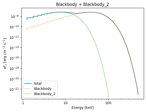
m8 = Blackbody(kT=kT1) + Blackbody(kT=kT2)
m8

Additive Model: Blackbody + Blackbody_2

No.	Component	Parameter	Value	Bound	Prior
1	Blackbody	kT	10	(0.1, 150)	Uniform(0.1, 150)
2	Blackbody	K	1	(1e-10, 1e+10)	Uniform(1e-10, 1e+10)
*	Blackbody_2	kT	f * Blackbody.kT
3	Blackbody_2	K	1	(1e-10, 1e+10)	Uniform(1e-10, 1e+10)
4		f	0.2	(0.01, 1)	Uniform(0.01, 1)

photon_egrid = np.linspace(1, 500.0, 1000)
egrid_mid = 0.5 * (photon_egrid[:-1] + photon_egrid[1:])
compiled_model = m8.compile()
vFv = compiled_model.eene(photon_egrid)
bb1 = compiled_model.eene(photon_egrid, params={'Blackbody_2.K': 0.0})
bb2 = compiled_model.eene(photon_egrid, params={'Blackbody.K': 0.0})
plt.step(egrid_mid, vFv, label='total')
plt.step(egrid_mid, bb1, ls=':', label='Blackbody')
plt.step(egrid_mid, bb2, ls=':', label='Blackbody_2')
plt.legend()
plt.title(m8.name)
plt.xlabel('Energy [keV]')
plt.ylabel(r'$\nu F_\nu$ [erg cm$^{-2}$ s$^{-1}$]')
plt.xscale('log')
plt.yscale('log')

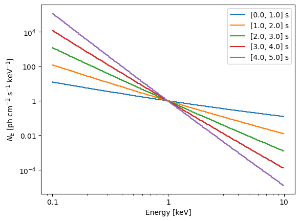
We can create a series of power-law models, whose photon indices are evolving from hard to soft,

# Create 10 time bins
n = 5
time_grid = np.linspace(0.0, 5.0, n + 1)

# The initial photon index
a0 = UniformParameter(
    name='a0',
    default=0.5,
    min=0.1,
    max=1.0,
)

# The decreasing rate of photon index
rate = UniformParameter(
    name='r',
    default=1.0,
    min=0.5,
    max=2.0,
)

models = []
for i in range(n):
    t = ConstantInterval('t', time_grid[i : i + 2])
    alpha = a0 + t * rate
    models.append(PowerLaw(alpha=alpha))
models[0]

Additive Model: PowerLaw

No.	Component	Parameter	Value	Bound	Prior
	PowerLaw	alpha	a0 + t * r
1	PowerLaw	K	1	(1e-10, 1e+10)	Uniform(1e-10, 1e+10)
2		a0	0.5	(0.1, 1)	Uniform(0.1, 1)
		t	[0, 1]
3		r	1	(0.5, 2)	Uniform(0.5, 2)

models[1]

Additive Model: PowerLaw

No.	Component	Parameter	Value	Bound	Prior
	PowerLaw	alpha	a0 + t * r
1	PowerLaw	K	1	(1e-10, 1e+10)	Uniform(1e-10, 1e+10)
2		a0	0.5	(0.1, 1)	Uniform(0.1, 1)
		t	[1, 2]
3		r	1	(0.5, 2)	Uniform(0.5, 2)

Note the a0 and r parameters are shared among models.

# Plot with default parameters values
photon_egrid = np.geomspace(0.1, 10.0, 300)
egrid_mid = 0.5 * (photon_egrid[:-1] + photon_egrid[1:])
for i in range(n):
    ne = models[i].compile().ne(photon_egrid)
    label = f'[{time_grid[i]}, {time_grid[i + 1]}] s'
    plt.step(egrid_mid, ne, label=label)
plt.legend()
plt.xlabel('Energy [keV]')
plt.ylabel('$N_E$ [ph cm$^{-2}$ s$^{-1}$ keV$^{-1}$]')
plt.xscale('log')
plt.yscale('log')

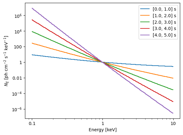
# Plot with a0=0, r=0.2
params = {'a0': 0, 'r': 1.5}
photon_egrid = np.geomspace(0.1, 10.0, 300)
egrid_mid = 0.5 * (photon_egrid[:-1] + photon_egrid[1:])
for i in range(n):
    ne = models[i].compile().ne(photon_egrid, params=params)
    label = f'[{time_grid[i]}, {time_grid[i + 1]}] s'
    plt.step(egrid_mid, ne, label=label)
plt.legend()
plt.xlabel('Energy [keV]')
plt.ylabel('$N_E$ [ph cm$^{-2}$ s$^{-1}$ keV$^{-1}$]')
plt.xscale('log')
plt.yscale('log')

When generating the alpha parameter for power-law model of each time slice, we set alpha = a0 + t * rate, rather than using the CompositeParameter. This is because ELISA provides a set of arithmetic operators to create CompositeParameter in a more straightforward way. We can use these operators on two parameters (including composite ones):

• +: sum

• -: subtraction

• *: multiplication

• /: division

• **: power

For example,

x = UniformParameter('x', 5, 1, 10)
y = UniformParameter('y', -2, -5, 10)
z = x**y
print(type(z).__name__, z)

CompositeParameter x^y

Manipulating Parameters of Components

We can manipulate the parameters of the components after the model is created.

m9 = PowerLaw()

# We first get the powerlaw component,
# then get K parameter of the component.
# Note that K is a UniformParameter by default,
# with five attributes: default, min, max, log, and fixed.

K = m9.PowerLaw.K
print('K', type(K).__name__, K.default, K.min, K.max, K.log, K.fixed, sep=', ')
m9

K, UniformParameter, 1.0, 1e-10, 10000000000.0, False, False

Additive Model: PowerLaw

No.	Component	Parameter	Value	Bound	Prior
1	PowerLaw	alpha	1.01	(-3, 10)	Uniform(-3, 10)
2	PowerLaw	K	1	(1e-10, 1e+10)	Uniform(1e-10, 1e+10)

# Modify the K parameter
m9.PowerLaw.K.default = 1.5
m9['PowerLaw'].K.min = 0.1
m9.PowerLaw['K'].max = 5.0
m9['PowerLaw']['K'].log = True
m9

Additive Model: PowerLaw

No.	Component	Parameter	Value	Bound	Prior
1	PowerLaw	alpha	1.01	(-3, 10)	Uniform(-3, 10)
2	PowerLaw	K	1.5	(0.1, 5)	LogUniform(0.1, 5)

# Set K to DistParameter with LogNormal distribution
m9.PowerLaw.K = DistParameter(
    name='K',
    dist=dist.LogNormal(10, 1),
    default=10,
)
m9

Additive Model: PowerLaw

No.	Component	Parameter	Value	Bound	Prior
1	PowerLaw	alpha	1.01	(-3, 10)	Uniform(-3, 10)
2	PowerLaw	K	10	Positive(lower_bound=0.0)	LogNormal(loc=10, scale=1)

A more convenient method to create a model with two blackbodies, as shown in the example above, can be as follows:

f = UniformParameter('f', 0.5, 0.01, 1.0)
m10 = Blackbody() + Blackbody()
m10.Blackbody_2.kT = f * m10.Blackbody.kT
m10

Additive Model: Blackbody + Blackbody_2

No.	Component	Parameter	Value	Bound	Prior
1	Blackbody	kT	3	(0.0001, 200)	Uniform(0.0001, 200)
2	Blackbody	K	1	(1e-10, 1e+10)	Uniform(1e-10, 1e+10)
*	Blackbody_2	kT	f * Blackbody.kT
3	Blackbody_2	K	1	(1e-10, 1e+10)	Uniform(1e-10, 1e+10)
4		f	0.5	(0.01, 1)	Uniform(0.01, 1)

Conclusion

The parameter interface of ELISA provides versatile approaches to configuring the parameters of model components. You can use parameters with default configuration, or create parameters with custom values, bounds, and priors. Additionally, linking parameters across various model components is supported.