A Quick Start Tutorial#

This tutorial provides a quick start guide to using ELISA to fit a spectral model to X-ray spectral data. The tutorial is divided into three sections:

Load Data and Define Spectral Model
Bayesian Fit
Maximum Likelihood Fit

The data used in this tutorial is from the Insight-HXMT observation of the Crab Nebula. The spectra are obtained by the Low Energy (LE), the Medium Energy (ME), and the High Energy (HE) telescopes. The spectral model used in this tutorial is a power-law model modified by a photoelectric absorption.

The tutorial demonstrates how to fit the spectral model to the data using both Bayesian and Maximum Likelihood methods.

Tip

By default, ELISA uses up to 4 CPU cores for parallel computation when available. To change the number of CPU cores in use, place the following at the beginning of your script:

import elisa
elisa.set_cpu_cores(8)  # Set to 8 CPU cores for example

1. Load Data and Define Spectral Model#

from elisa import BayesFit, Data, MaxLikeFit
from elisa.models import PhAbs, PowerLaw

LE = Data(
    erange=[1.5, 10],
    specfile='data/P011160506306_LE_TOTAL.fits',
    backfile='data/P011160506306_LE_BKG.fits',
    respfile='data/P011160506306_LE_RSP.fits',
    group='opt',
)

ME = Data(
    erange=[10, 35],
    specfile='data/P011160506306_ME_TOTAL.fits',
    backfile='data/P011160506306_ME_BKG.fits',
    respfile='data/P011160506306_ME_RSP.fits',
    group='opt',
)

HE = Data(
    erange=[28, 250],
    specfile='data/P011160506306_HE_TOTAL.fits',
    backfile='data/P011160506306_HE_BKG.fits',
    respfile='data/P011160506306_HE_RSP.fits',
    group='opt',
)

data = [LE, ME, HE]

model = PhAbs() * PowerLaw()

/home/docs/checkouts/readthedocs.org/user_builds/astro-elisa/conda/latest/lib/python3.12/site-packages/elisa/util/config.py:82: Warning: only 2 CPUs available, will use 1 CPUs
  warnings.warn(msg, Warning)

/tmp/ipykernel_3288/1226189312.py:12: Warning: spectrum data/P011160506306_ME_BKG.fits has zero statistical errors, which may lead to wrong result under Gaussian statistics, consider grouping the spectrum
  ME = Data(
/tmp/ipykernel_3288/1226189312.py:20: Warning: spectrum data/P011160506306_HE_BKG.fits has zero statistical errors, which may lead to wrong result under Gaussian statistics, consider grouping the spectrum
  HE = Data(

2. Bayesian Fit#

fit = BayesFit(data, model)
fit

Bayesian Fit

Data	Model	Statistic
LE	PhAbs * PowerLaw	pgstat
ME	PhAbs * PowerLaw	pgstat
HE	PhAbs * PowerLaw	pgstat

No.	Component	Parameter	Value	Prior
1	PhAbs	nH	1	Uniform(0, 1e+06)
2	PowerLaw	alpha	1.01	Uniform(-3, 10)
3	PowerLaw	K	1	Uniform(1e-10, 1e+10)

Run the No-U-Turn Sampler#

posterior = fit.nuts(chains=4, progress=False)
posterior

/home/docs/checkouts/readthedocs.org/user_builds/astro-elisa/conda/latest/lib/python3.12/site-packages/elisa/infer/fit.py:833: UserWarning: There are not enough devices to run parallel chains: expected 4 but got 1. Chains will be drawn sequentially. If you are running MCMC in CPU, consider using `numpyro.set_host_device_count(4)` at the beginning of your program. You can double-check how many devices are available in your system using `jax.local_device_count()`.
  sampler = MCMC(

Posterior Result

Parameters

Parameter	Mean	StdDev	Median	68.3% Quantile	ESS	Rhat
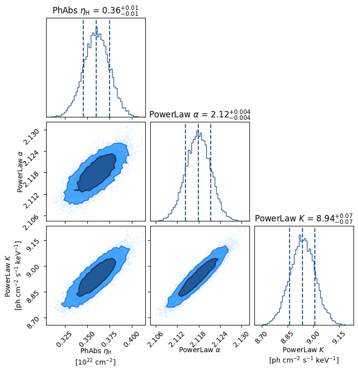
PhAbs.nH	0.36	0.0146	0.36	[-0.0145, 0.0147]	8072	1.00
PowerLaw.alpha	2.12	0.0035	2.12	[-0.00353, 0.00352]	9123	1.00
PowerLaw.K	8.94	0.0734	8.94	[-0.0739, 0.0724]	8155	1.00

Statistics

Data	Statistic	Mean	Median	Channels
LE	pgstat	95.53	95.03	80
ME	pgstat	8.00	7.74	16
HE	pgstat	43.89	43.56	25
Total	stat/dof	147.43/118	146.81/118	121

Information Criterion

Method	Deviance	p
LOOIC	149.96 ± 19.56	2.40
WAIC	149.93 ± 19.56	2.38

Pareto k Diagnostic

Range	Flag	Count	Pct.
(-Inf, 0.70]	good	121	100.0%
(0.70, 1]	bad	0	0.0%
(1, Inf)	very bad	0	0.0%

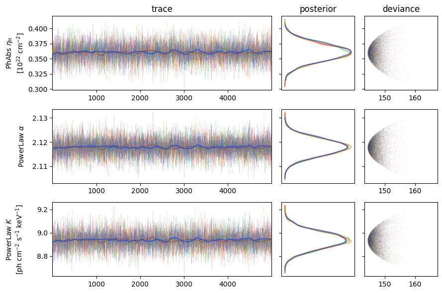
Plot the Trace of Sampler#

fig = posterior.plot.plot_trace()

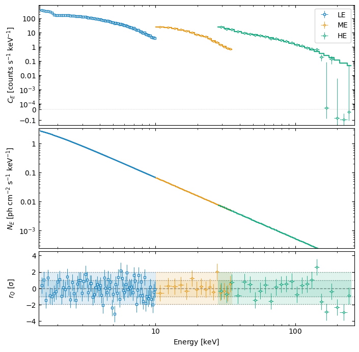
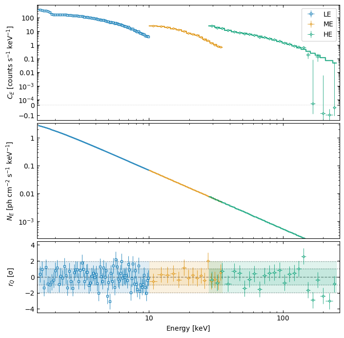
../_images/a58f5e9e8a1b9898679e4c1febf6d632c603b4c158253b02ab35997d2a00ef14.png

Plot of Spectral Fit and Residuals#

fig = posterior.plot()

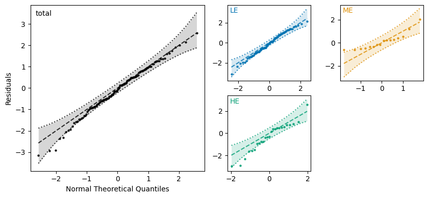
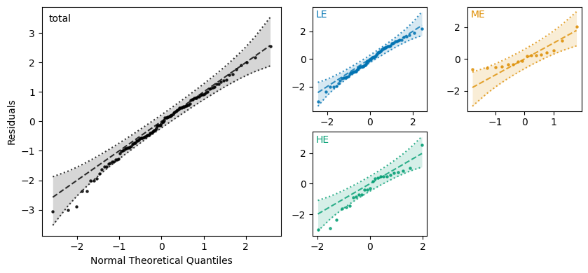
../_images/1adf73426c4704b4b36ac161bda42b79edabfd9213474949cc454600128a80a7.png

Goodness of Fit: Quantile-Quantile Plot#

fig = posterior.plot.plot_qq(detrend=False)

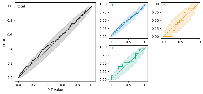
../_images/a1c1b78bdd6ebbd2bfc3535053c32450ec3798fc64782535a02a109746efefd1.png

Goodness of Fit: Probability Integral Transform ECDF Plot#

fig = posterior.plot.plot_pit(detrend=False)

../_images/0c2b250aa7cc316ec1cd8e449f272c1fd37871950afd5b44e7c4912e779b522d.png

Plot Marginal Posterior Distribution#

fig = posterior.plot.plot_corner()

../_images/d0d3789a615b2a77e73ea0c1c29844cda1ea0658c0f9b0bbfb619ef9850448a3.png

Calculate Credible Intervals of Parameters#

ci = posterior.ci()
ci

CredibleInterval(median={'PhAbs.nH': 0.3603830205638544, 'PowerLaw.alpha': 2.117877468077268, 'PowerLaw.K': 8.936866949299617}, intervals={'PhAbs.nH': (0.3458840053593828, 0.3750691150358259), 'PowerLaw.alpha': (2.1143515675068483, 2.1213933564573035), 'PowerLaw.K': (8.862981386384684, 9.009236407669906)}, errors={'PhAbs.nH': (-0.01449901520447161, 0.0146860944719715), 'PowerLaw.alpha': (-0.003525900570419793, 0.00351588838003547), 'PowerLaw.K': (-0.07388556291493309, 0.07236945837028941)}, cl=np.float64(0.6826894921370859), method='ETI', dist={'PhAbs.nH': array([[0.36018297, 0.35964464, 0.35693911, ..., 0.36456697, 0.36582168,
        0.36311594],
       [0.3782076 , 0.36736489, 0.36024446, ..., 0.37805725, 0.3675747 ,
        0.36654078],
       [0.3668114 , 0.36643217, 0.37302283, ..., 0.34919229, 0.35134318,
        0.34670359],
       [0.33436351, 0.33300345, 0.36104852, ..., 0.40294949, 0.40196613,
        0.388544  ]], shape=(4, 5000)), 'PowerLaw.alpha': array([[2.12211822, 2.12012776, 2.11891948, ..., 2.1144305 , 2.12192537,
        2.11605011],
       [2.11896715, 2.12088983, 2.11705767, ..., 2.11970716, 2.11886832,
        2.11651229],
       [2.11588473, 2.11534243, 2.11777053, ..., 2.11677855, 2.11953614,
        2.11594131],
       [2.11241539, 2.11071551, 2.12012529, ..., 2.12619398, 2.12527212,
        2.12198885]], shape=(4, 5000)), 'PowerLaw.K': array([[8.98768314, 9.00855438, 8.93705757, ..., 8.91995767, 8.97766524,
        8.91558281],
       [9.00408312, 9.000614  , 8.9461778 , ..., 9.01225573, 8.94548567,
        8.94059428],
       [8.91232557, 8.91605017, 8.92972885, ..., 8.92147757, 8.92075066,
        8.90559839],
       [8.81699128, 8.77282012, 8.9560633 , ..., 9.13299799, 9.12103654,
        9.0373675 ]], shape=(4, 5000))})

ci.median

{'PhAbs.nH': 0.3603830205638544,
 'PowerLaw.alpha': 2.117877468077268,
 'PowerLaw.K': 8.936866949299617}

ci.errors

{'PhAbs.nH': (-0.01449901520447161, 0.0146860944719715),
 'PowerLaw.alpha': (-0.003525900570419793, 0.00351588838003547),
 'PowerLaw.K': (-0.07388556291493309, 0.07236945837028941)}

3. Maximum Likelihood Fit#

model.PhAbs.nH.default = 0.35
fit2 = MaxLikeFit([LE, ME, HE], model)
fit2

Maximum Likelihood Fit

Data	Model	Statistic
LE	PhAbs * PowerLaw	pgstat
ME	PhAbs * PowerLaw	pgstat
HE	PhAbs * PowerLaw	pgstat

No.	Component	Parameter	Value	Bound
1	PhAbs	nH	0.35	(0, 1e+06)
2	PowerLaw	alpha	1.01	(-3, 10)
3	PowerLaw	K	1	(1e-10, 1e+10)

Use Levenberg-Marquardt algorithm to find the MLE#

mle = fit2.mle(method='lm')
mle

MLE Result

Parameters

Parameter	MLE	Error
PhAbs.nH	0.36	0.01467
PowerLaw.alpha	2.118	0.00352
PowerLaw.K	8.935	0.0739

Fit Statistics

Data	Statistic	Value	Channels
LE	pgstat	93.61	80
ME	pgstat	7.60	16
HE	pgstat	43.26	25
Total	stat/dof	144.48/118	121

Information Criterion

Method	Value
AIC	150.68
BIC	158.87

Fit Status

Migrad
FCN = 144.5 (χ²/ndof = 1.2)	Nfcn = 76
EDM = 6.49e-10 (Goal: 0.0002)	time = 0.7 sec
Valid Minimum	Below EDM threshold (goal x 10)
No parameters at limit	Below call limit
Hesse ok	Covariance accurate

Plot of Spectral Fit and Residuals#

fig = mle.plot()

../_images/ff9ac75ffce1c6c27768eb2f07306223d84f6f6f925b3089f75462a0faf9ac6e.png

Goodness of Fit: Quantile-Quantile Plot#

fig = mle.plot.plot_qq(detrend=False)

../_images/38d927d3f56b56d133f613292edd8cac02f5d71e983d5b14841018a070324abf.png

Goodness of Fit: Probability Integral Transform ECDF Plot#

fig = mle.plot.plot_pit(detrend=False)

../_images/138e86b1b341d8fc9f21a93cdd9ff83bcef455ee4c37205574907e964216506f.png

Calculate Confidence Intervals of Parameters#

ci = mle.ci()
ci

ConfidenceInterval(mle={'PhAbs.nH': 0.35997081629801786, 'PowerLaw.alpha': 2.117804642738316, 'PowerLaw.K': 8.9349475334073}, se={'PhAbs.nH': 0.014673851513267541, 'PowerLaw.alpha': 0.0035202870609333642, 'PowerLaw.K': 0.07390147136562786}, intervals={'PhAbs.nH': (0.3453066679006991, 0.37465441667999444), 'PowerLaw.alpha': (2.114290122134887, 2.1213307115596707), 'PowerLaw.K': (8.861387983032087, 9.00919350394845)}, errors={'PhAbs.nH': (-0.014664148397318777, 0.01468360038197658), 'PowerLaw.alpha': (-0.003514520603428828, 0.0035260688213547553), 'PowerLaw.K': (-0.07355955037521333, 0.0742459705411509)}, cl=np.float64(0.6826894921370859), method='profile', status={'PhAbs.nH': {'valid': (True, True), 'at_limit': (False, False), 'at_max_fcn': (False, False), 'new_min': (False, False)}, 'PowerLaw.alpha': {'valid': (True, True), 'at_limit': (False, False), 'at_max_fcn': (False, False), 'new_min': (False, False)}, 'PowerLaw.K': {'valid': (True, True), 'at_limit': (False, False), 'at_max_fcn': (False, False), 'new_min': (False, False)}})

ci.mle

{'PhAbs.nH': 0.35997081629801786,
 'PowerLaw.alpha': 2.117804642738316,
 'PowerLaw.K': 8.9349475334073}

ci.errors

{'PhAbs.nH': (-0.014664148397318777, 0.01468360038197658),
 'PowerLaw.alpha': (-0.003514520603428828, 0.0035260688213547553),
 'PowerLaw.K': (-0.07355955037521333, 0.0742459705411509)}